DHARMa – an R package for residual diagnostics of GLMMs

I just released a small R package that I have been working on for a while. The motivation for this package came from the observation that I kept on receiving questions about residual checks for GLMMs. The problem that people have is that they have fitted their GLMM, maybe they tested it for overdispersion and potentially corrected that, and now they plot their residuals and get something like this:

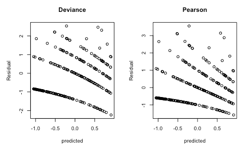
Deviance and Pearson residuals for a correctly specified Poisson GLMM

Is there a pattern that shows a dependence of residuals on the predicted value? Are the distributional assumptions of the fitted model correct? People are often concerned when they see plots such as the above because they learned in their elementary stats classes that residuals should look homogeneous. Well, that is the case for LMs, but not for GLMMs. When you work a bit more with GLMMs, you learn that inhomogeneous Pearson residuals are not necessarily a reason for concern. But even so, it is hard to tell if a GLMM is misspecified, just from looking at Pearson or deviance residuals.

The solution to this problem is well known, but a bit tricky to implement, which is presumably why it is seldom used. The goal of DHARMa is to change this and make residual checks for GLMMs as straightforward as for LMs.

The recipe is the following: for your fitted GLMM

1. Simulated many new datasets with the model assumptions and the fitted parameters
2. Define the residual for each observation as the proportion of the simulated observations that are lower than the observed value (see figure below)

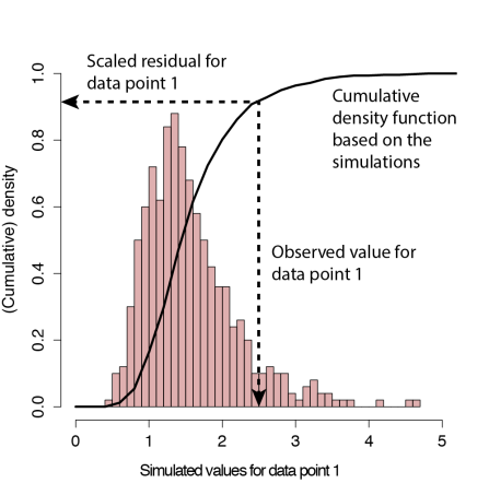
Definition of the scaled residual for data point 1, aka quantile residuals, aka the little sister of the Bayesian p-value. Simulations are performed with the fitted point estimate. The latter is the difference to Bayesian p-values, where the cumulative density of the posterior predictive distribution is used.

 

The resulting residuals (sometimes called quantile residuals) are scaled between 0 and 1. What is more important however, is that we have good theory about how they should be distributed. If the model is correctly specified, then the observed data can be thought of as a draw from the fitted model. Hence, for a correctly specified model, all values of the cumulative distribution will appear with equal probability. What that means is that we expect the distribution of the residuals to be flat, regardless of whether we have a Poisson, binomial or another model structure (see, e.g., Dunn & Smyth, 1996; Gelman & Hill. 2006).

Thus, you can simply plot your residuals, and if you see a pattern in the residuals, or the distribution is not uniform, then there is a problem in the model. To give an example: the plot below shows the DHARMa standard residual plots for a Poisson GLMM with underdispersion. The underdispersion problem shows up as a deviation from uniformity in the qq plot, and as an excess of residual values around 0.5 in the residual vs. predicted plots.

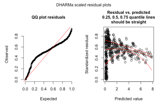
An example of a DHARMa residual plot for an underdispersed Poisson GLMM

That’s it basically. When we go into the details, there are a few further considerations. One is that the DHARMa package adds some noise to create continuous residual distributions for integer-valued responses such as Poisson or binomial. The other is that one can decide if new data is simulated conditional on the fitted random effects, or unconditional. The difference between the two is that for the first option, you look at whether your observed data is compatible with the model assumptions, conditional on the random effects being at their estimated values, while the second options re-simulates random effects and therefore implicitly tests their assumptions as well. I recommend to give it some thought which of your random effects you want to keep constant in the simulations. Some more hints are in the vignette.

The package also includes some dedicated test functions for

• Over/underdispersion
• Zero-inflation
• Residual temporal autocorrelation
• Spatial temporal autocorelation

Hence, no excuse any more to not check either of those for your fitted GLMMs. What is missing still are some dedicated tests of the random-effect structure. I’m planning to add this in the future.

p.s.: DHARMa stands for “Diagnostics for HierArchical Regression Models” – which, strictly speaking, would make DHARM. But in German, Darm means intestines; plus, the meaning of DHARMa in Hinduism makes the current abbreviation so much more suitable for a package that tests whether your model is in harmony with your data:

From Wikipedia, 28/08/16: In Hinduism, dharma signifies behaviours that are considered to be in accord with rta, the order that makes life and universe possible, and includes duties, rights, laws, conduct, virtues and ‘‘right way of living’’.

References

1. Hartig, F. (2016). DHARMa: residual diagnostics for hierarchical (multi-level/mixed) regression models. R package version 0.1. 0. CRAN / GitHub
2. Dunn, K. P., and Smyth, G. K. (1996). Randomized quantile residuals. Journal of Computational and Graphical Statistics 5, 1-10.
3. Gelman, A. & Hill, J. Data analysis using regression and multilevel/hierarchical models Cambridge University Press, 2006