This (co-)guest post by Carsten F. Dormann & Florian Hartig summarizes a comprehensive review on model averaging for predictive inference, just published in Ecological Monographs.
Dormann, C.F., Calabrese, J.M., Guillera-Arroita, G., Matechou, E., Bahn, V., Bartoń, K., et al. (in press). Model averaging in ecology: a review of Bayesian, information-theoretic and tactical approaches for predictive inference. Ecol Monogr, doi: 10.1002/ecm.1309
When times are dire, and data are scarce, quantitative ecologists (or quantitative scientists in general) often reach into their quiver for an arrow called model averaging.
Model averaging refers to the practice of using several models at once for making predictions (the focus of our review), or for inferring parameters (the focus of other papers, and some recent controversy, see, e.g. Banner & Higgs, 2017). There are literally thousands of publications across the disciplines that practice “classical” model averaging, i.e. averaging a few or many models that one could also use “stand-alone”. Additionally, model averaging, as a principle, underlies many of the most commonly used machine-learning methods (e.g. as bagging of trees in random forest or of neural network predictions). We only devoted a few sentences in the appendix of the paper to this, but we think that the link between classical model averaging and machine learning is not sufficiently appreciated and could be further explored.
In ecology, averaging of statistical models is heavily dominated by the “information-theoretical” framework popularised by Burnham & Anderson (2002), while alternative methods that are used in other scientific fields are less well-known. When we set out in March 2015, in the form of a workshop, to conduct a comprehensive review of the wealth of model-averaging approaches, we anticipated this diversity, but not the road full of potholes that we encountered. Studies and information about the topic are fragmented across disciplines, many of which have developed their own ideas and terminology to approach the model-averaging problem. Moreover, the field is largely characterized by a hands-on approach, where alternative ways to average and quantify uncertainties are proposed in abundance; however, with very little “cleaning up” of what works and what doesn’t. As a consequence, what started as a small workshop developed into a multi-author, multi-year activity that culminated in a multi-facetted publication, in which the actual technical description of the various available model-averaging algorithms is only one part.
Apart from mapping the method jungle, our review explains, at least in ecology probably for the first time,
- why and when model averaging works, and what this depends on (see our explanation of how bias, (co)variance and uncertainty of weight estimation influence the benefits of MA);
- how to quantify the uncertainty of model-averaged predictions, and why there are substantial problems to achieve good uncertainty estimates.
The goal of this post is to wet your appetite, not to reproduce the entire paper. Thus, in what follows, we will only have a superficial look at the ingredients of each of these points.
Bias, (co)variance and weight uncertainty
The first part of our paper shows how error of model-averaged predictions can be decomposed into bias and error (co)variance of the contributing models, and uncertainty of weight estimation. Some key insights are:
- If our different models err systematically, but equally on the high and the low side, then their average has less bias.
- If our models vary stochastically, but all in the same way, then there is little point in averaging them. MA becomes more useful the lower the covariance between estimates.
- If all our models are more or less great (or poor), we can save us the trouble of estimating weights.
Here are some titbits of explanation:
First off, the prediction uncertainty, quantified e.g. as mean squared error MSE, is the sum of squared bias and variance. Hence, we can decompose the effect of model averaging into its effect on bias, and on variance.
The first point about systematic error is usually not so relevant for statistical models. Classical/typical/good statistical models are unbiased, i.e. their mean prediction does not deviate from the truth. For process-based models, this need not be the case. If a processes is specified wrongly, the model’s predictions may be consistently too high or too low. Averaging predictions from different process models, with biases in either way, should therefore cancel to some extent and hence reduce bias in the averaged prediction, explaining why model averaging is popular in process-based modelling communities such as climate modelling.
The second point about variance is more relevant for statistical models. Variance refers to the fact that an ideal statistical model gets it right on average (no bias), but will still make an error in each single application (variance). For an unbiased model, predictions will have a smaller error if their variance is lower. We show that, as a consequence of error propagation, the variance of the averaged prediction depends on the variance of each contributing model, as well as the co-variances among these predictions. Thus, if all models made identical predictions, the covariance would cancel any benefit of averaging variances. If, however, model predictions are perfectly uncorrelated, we get great benefits for their prediction’s variance.
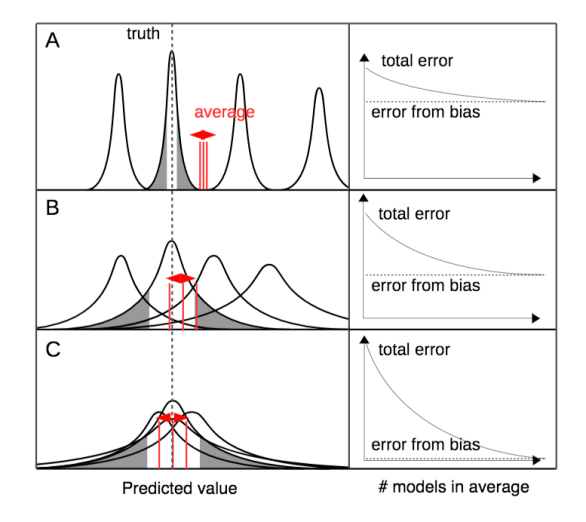
Fig. 1 from Dormann et al. – conceptual depiction of the contributions of error to model averaging.
Hang on!? So if my models make very different predictions (which might be worrying for some), only then I get the full benefits of model averaging? Correct!
And it gets more complicated.
There is another factor influencing the variance, which is the weighting of the models. If we threw all models we can get our hands on willy-nilly into an averaging procedure, then surely, we need to sort the wheat from the chaff first. It seems illogical to allow a crappy model to ruin our model average, so we need to downweigh it. Or, as the advice in many papers reads: “Only average plausible models.”
Here, it gets really confusing in the literature, because that’s exactly what many highly successfully machine-learning approaches do not do. For example, in bagging, a commonly used machine learning principle, all models are averaged, and they are not even weighted!
The underlying issue is that, when estimating model weights, we may accrue substantial uncertainty, and this uncertainty also propagates into our model-averaged prediction (Claeskens & al. 2016)! Indeed, it may often be wiser not to compute model weights, if we already have pre-selected our models, as is the common procedure in economics and with the IPCC earth-system-models.
How uncertain is the model-averaged prediction?
After having established that model averaging can (in the right circumstances) improve predictions, let us turn to the second presumed benefit of model averaging, a better representation of uncertainty.
A commonly named reason to use model averaging is that we cannot decide which of our candidate models is the correct one, and therefore want to include them all to better represent our structural uncertainty. So then the obvious question is: how do we compute an uncertainty estimate of a model average? As ingredients we (possibly) have (a) a prediction from each model, (b) a standard error for each model’s prediction, e.g. from bootstrapping, (c) the model weights, and (d) the unknown uncertainty in the model weights. How to brew them into one 95% confidence interval of the model-averaged prediction?
Again, we shall not disclose the details as given in the paper, but this issue caused some serious head-scratching among the authors (each by herself, of course).

As a teaser: there are a few proposals of how to construct frequentist confidence intervals, but they are by-and-large problematic. Some assume perfect correlation of predictions and “non-standard mathematics”, others assume perfect independence and work surprisingly well in our little test-run. (Our personal all-time favourite, the full model, did of course best, but that is not a very helpful finding for any process modeller.)
However, it should be noted that things are not so bad if one is only interested in a predictive error (which can be obtained by cross-validation), or if one works Bayesian, as posterior predictive intervals are more naturally to compute.
How to compute the model-averaging weights?
Finally, we come to the topic that you all must have waited for: what’s the best method to compute the weights? We gave it away already: it’s hard to say, because there are many proposals out there, far more than informative method comparisons.
We divided the method-zoo into three sections: one for Bayesians, one for “IC folks”, and one for practically-oriented folks (aka machine learners & co).
The pure Bayesian side is theoretically simple, but difficult implementation-wise (we’re talking here about the problem of estimating marginal likelihoods of the models, e.g. by reversible-jump MCMC or some other approximations).
The information theoretical approaches are theoretically somewhat more dubious (because they seem to strongly head into the Bayesian direction, with model weights being something akin to model probabilities, but then verbally shun Bayesian viewpoints), but well established computationally.
The smorgasbord (this word was chosen to reflect the European dominance in the author collective) of approaches not fitting either category, which we labelled tactical, comprised the sound and obscure. In short, we summarize here all the approaches that directly target a reduction of predictive error, be it by machine-learning principles or verbal argument. Key examples here are stacking and jackknife model averaging.
Detailed explanations of each approach are given in the paper, and we also ran most methods through two case studies. We found little in our results to justify the dominance of AIC-based model averaging. And model-averaging did not necessarily outperform single models.
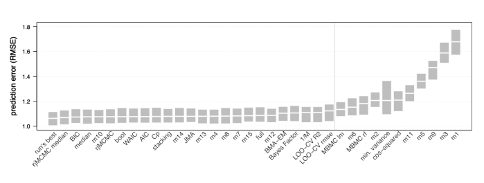
Fig. 5 from Dormann et al. – Performance of different methods in a case study
Take-home message
Model averaging has no super-powers. Claims of “combining the best from all models” are plain nonsense. Like most other statistical methods, at close inspection, we see that model averaging has benefits and costs, and an analyst must weigh them carefully against each other to decide which approach is most suitable for their problem.
Benefits include a possible reduction of predictive error. Costs include the fact that this does not always work. And that confidence intervals (and also p-values) are difficult to provide.
To reduce prediction error, we recommend cross validation-based approaches, which are specifically designed to achieve this goal. Embracing model structural uncertainty is certainly a laudable ambition, but the precise mathematics are complicated, and robust methods that work out of the box are not yet worked out.
Literature
Banner, K. M. and M. D. Higgs (2017) Considerations for assessing model averaging of regression coefficients. Ecological Applications, 28:78–93.
Burnham KP, Anderson DR (2002) Model Selection and Multi-Model Inference: a Practical Information-Theoretical Approach. 2nd ed. Berlin: Springer.
Claeskens G, Magnus JR, Vasnev AL, Wang W. The forecast combination puzzle: A simple theoretical explanation. International Journal of Forecasting. 2016;32:754–62.
Dormann, C.F., Calabrese, J.M., Guillera-Arroita, G., Matechou, E., Bahn, V., Bartoń, K., et al. (in press). Model averaging in ecology: a review of Bayesian, information-theoretic and tactical approaches for predictive inference. Ecol Monogr, doi: 10.1002/ecm.1309


Carsten and Florian — this is a fantastic summary (and teaser) of the review. I’m following up on our e-mail exchange on a matter that is only supplemental (literally) to the paper — your argument that “For non-linear models, such as GLMs with log or logit link functions g(x), such coefficient averaging is not equivalent to prediction averaging” on p.2 of the supplement. For GLMs, this seemed obviously wrong to me when I read it and I initially thought it was because the LHS of equation S2 was wrong because the averaging was on the response scale. But from our discussion, I learned that you believe it is the RHS that is wrong. So, our differences can be summarized as (a longer version with some code is here)
1. The papers argue that predictions should be computed on the link scale, back-transformed to the response scale, and then averaged on the response scale. From our e-mail exchange, I infer that the reasons for averaging on the response scale are first, everyone outside of ecology does it, and second, predictions have to be averaged on the response scale for non-linear models because there is no link scale, and, since, GLMs are non-linear, they should be averaged on the response scale.
2. I assumed that because a GLM model is fit on a linear scale, any subsequent averaging should be on the linear scale. My reason is that because a GLM is a linear model, additive math should be additive (on the link scale) and not multiplicative (on the response scale) to be consistent with the meaning of the fit parameters. For example, a prediction is a weighted sum of the data, with weights that are a function of a linear fit, and everyone agrees that predictions should be computed on the link scale and then back-transformed (if desired). And, a model-averaged prediction is a weighted sum, with both weights and variables that are functions of linear fits, and so the predictions should be averaged on the link scale, and then back-transformed to the response scale (if desired).
My assumption was exactly that, since I don’t either model-average or use GLMs in my own work. But I checked my assumption with MuMIn, which averages on the link-scale, which agrees with my way thinking about this. After our e-mail exchange, I also googled around and found that Russell Lenth in his excellent emmeans package computes marginal means of GLMs on the link scale before back-transforming to the response scale, and his reasons are those of mine:
However – Like MuMIn, the default prediction of version 1.4.9 of BAS (Bayesian model averaging) outputs the model-averaged prediction on the link scale (RHS of S2) in the value $Ybma. BUT, unlike MuMIn, the prediction on the response scale, in the value $fit, is not exp(Ybma) but the predictions re-averaged on the response scale. I find this weird — if the default prediction is averaged on the link scale and I want to interpret this on the response scale, then I would just back-transform the default rather than re-averaging the back-transformed predictions. This would be like recomputing the predictions by first back-transforming the coefficients to the response scale. It could also lead to lack of reproducibility.
Perhaps this is all academic. As the supplement p.2 notes and in my simulations with either a logistic or poisson link function with the simple models that I simulated, the difference in the predictions between the LHS and RHS of ea. S2 is trivially small (at least relative to other sources of error), but maybe there are important cases where this isn’t so — again, I’m not experienced in this area.
LikeLike
Hi Jeff, thanks for your comments and your interest in our review.
Just to back up for other readers, we’re speaking about supplement S1, eq. S2, where we state that, if parameters affect the model output nonlinearly, then the average of the predictions is not the same as the prediction with the average of the parameters
This is also discussed in Burnham & Anderson 2002, 2nd ed., page 153, and simply a mathematical fact (it’s basically Jensen’s inequality).
What does that tell us for GLMs? Burnham & Anderson unfortunately didn’t name GLMs explicitly, but of course, due to the nonlinear link function, this comment extends to GLMs. In that context, I’d like to comment on some of your statements: no, a GLM is NOT a linear model. Also, GLMs are NOT fit at the linear scale (at least according to my definition of “fit”), and I don’t see any support for your assertion that “everyone agrees that predictions should be computed on the link scale and then back-transformed (if desired)”. For me, I would conclude firstly that it’s a mathematical fact that
What we have learned so far is that we have two (non-equivalent) options for making predictions i) directly average predictions ii) average parameters and make predictions with the parameter average. Both of these options will in general differ, and the questions is of course which is better.
I appreciate that we do not deliver a constructive proof against option ii), but in general, I think it’s quite easy to construct counterexamples that show that ii) is a bad idea, or at least doesn’t improve over option i). Let me give you four approximate reasons though:
In conclusions, I don’t believe that there is much reason to think that the parameter average is more useful than the prediction average to make predictions.
Whether the parameter average is useful for other purposes (e.g. as an estimator for the effect of each predictor) is another question. We are working on a publication to comment on that, but I would not want to get into this discussion here.
LikeLike
Hi Florian, thanks for the response. I think there is continued miscommunication on what I’ve written that is stemming from the ambiguity of the phrase “averaged predictions”. A prediction can be averaged two ways 1) compute the predictions on the link scale for all models, average these on the link scale, back-transform if desired and 2) compute predictions on the link scale for all models, back transform predictions from all models to response scale, average on the response scale. #1 is not averaging the parameters, it is averaging predictions, although it is equivalent to averaging the parameters and then computing predictions mathematically.
1) You state “GLMs are NOT fit at the linear scale (at least according to my definition of “fit”)” You are correct that my language was ambiguous, the MSE is computed from g^-1(Xb) not Xb and in that sense the model is not fit on a linear scale. My point is that Xb is a *linear* predictor and I am arguing that additive relationships using this predictor (such as averages of Xb) should be additive to be consistent with the coefficients as the weights of a linear model.
2) You state “I don’t see any support for your assertion that ‘everyone agrees that predictions should be computed on the link scale and then back-transformed (if desired)’ ” in a GLM, E(Y) = mu = g^-1(Xb) yes? This is even in the parentheses of the LHS of eq. S2 above. These predictions (Xb) are computed on the link scale and then back transformed, if desired. I cannot see how this is controversial. I am not referring to model averaged predictions.
3) For a set of M models, there are M sets of (Xb) and M sets of their back-transformed values g^(-1)(Xb). Both sets are equally optimal because they are the same thing – just simple transformations of each other. Why is averaging g^(-1)(Xb) over the M sets more optimal than averaging (Xb) over the M sets and then back-transforming the averages? Or, restated, why is
mean[g^(-1)(Xb)] more optimal than g^(-1)(mean(Xb))
LikeLiked by 1 person
I also meant to ask if you could provide a short script generating a fake data set where mean[g^(-1)(Xb)] differs radically from g^(-1)(mean(Xb)). I’m not doubting this exists, I just don’t know how to generate it without just randomly searching.
LikeLiked by 1 person
Hi Jeff,
OK, with the comment on averaging predictions at the link scale, I now understand a bit better where you’re coming from. Note though that averaging at the scale of the linear predictor is mathematically identical to predicting with the average of the parameters. So, all my comments above apply identically to “averaging at the link scale”.
About 1/2: 1) OK 2) sorry, I thought you were referring to the averaged predictions
About your question 3: “Why is averaging g^(-1)(Xb) over the M sets more optimal than averaging (Xb) over the M sets and then back-transforming the averages?” – I think I have not much to add to my comments 1-4 above.
If none of this convinces you, I guess it boils down to just running the simulations. From our simulations, I can say that differences are usually not massive, but neither is there any sign that averaging the parameters creates better predictions. If you want to create strong differences between the two options, you have to create a lot of variance between the parameter estimates of the different models (to get Jensen’s inequality going). That will happen mostly if you have strong collinearity. I’m sorry, I can’t share my simulations right now because, as I said, we are working on a related publication.
LikeLiked by 2 people
Jeffrey, just to clarify: MuMIn’s `predict` can either average predictions on the response scale or link scale (which one is the default depends on the component models’ default prediction type), and the latter can be back-transformed. This is controlled by arguments `type` (“link” or “response”) and `backtransform`.
LikeLiked by 1 person
Kamil – thank you for the clarification and let me say the MuMIn functions are very straightforward to implement. The default prediction for glm is the response on the link scale. So the default model-averaged prediction in MuMIn for a glm object is the predictions averaged on the link scale, yes? I have argued (unsuccessfully) that this makes sense but I think the worry or criticism from Florian is that averaging on the link scale is not correct. So there may be criticism (not from me) of this statement in the MuMIn documentation “if [backtransform=]TRUE, the averaged predictions are back-transformed from link scale to re- sponse scale. This makes sense provided that all component models use the same family, and the prediction from each of the component models is calcu lated on the link scale.”
LikeLike
Argh – I’ve just been playing about with confidence intervals, as I was puzzled with AICcmodavg did not include them, and thought that model averaged confidence intervals – http://rpubs.com/jebyrnes/aic_prediction – were reasonable. Back to the drawing board? And/or is there a push to incorporate this thinking into that package, as it’s fairly widely used?
LikeLike
Hi Jarrett – my spontaneous reaction, skimming your script and the functions used there, is
1) It seems to me that AICcmodavg::modavgPred aims at calculating confidence intervals – you interpret the output as providing prediction intervals? Reading on, I was wondering if we’re on the same page about what the difference is between the confidence interval and the prediction interval https://en.wikipedia.org/wiki/Prediction_interval of a prediction?
2) The help says that AICcmodavg::modavgPred calculates the confidence interval of the prediction based on “[…] the classic computation based on asymptotic normality of the estimator […]”, but I’m not sure what that means exactly. As we discuss in our review, calculating CIs for the averaged predictions is in general a really wicked problem. In your script, it looks as if the CIs calculate by AICcmodavg::modavgPred are fairly wide, or a lot wider than the single model? This is not what I would have expected with the usual methods, unless we are speaking about what we call “mixing” (see below Fig. 3 from our review, which compares several methods to calculate CIs). I guess you would have to look a the code to see how they are calculated, or ask the developer Marc Mazerolle. I’ll drop him a line in case he cares to comment.
LikeLike
Florian,
Thanks for your response. I was thinking of confidence intervals of fit (which does not incorporate residual uncertainty) versus prediction intervals (which do). Sorry if this wasn’t clear from my writeup. modavgPred does the former, not the latter. Which I think is somewhat problematic for some real-world applications. The Baysian analysis in the middle bit hits at the difference in width of the two intervals. And my attempt at the end – weighted prediction intervals – was my attempt at a solution, and hence the extra width there.
Is that clearer?
Perhaps I have missed what y’all were getting at, but, I admit, I’m sitting in a workshop (where amusingly while I write this comment, we’re talking about model averaging for occupancy models) so have not fully read the paper.
LikeLike
(Also the class is excellent – the discussion got me curious to check back here – I’m not being the bad kid in the back of class! I swear!)
LikeLike
Hi Jarret – I see the question of whether to provide confidence and prediction intervals as perpendicular to both the MA and the Bayesian/Frequentist thing. Generally, we have two options:
i) The uncertainty about the mean prediction is given by the frequentist CI / Bayesian credible interval
ii) The uncertainty of a new measurement = i) + error term is the frequentist prediction interval, or the Bayesian equivalent, the posterior predictive simulation
There are some differences between the frequentist / Bayesian versions of i)/ii), but when running an lm or glm, those are usually negligible. And of course, the prediction interval ii) (or Bayesian equivalent) is always wider than the confidence interval i).
The question is now to take these two things over to a MA world. What we show in our review for the CI is that it’s quite hard to construct MA CIs that achieve nominal coverage. The same is true for Bayesian CIs, but Bayesian fundamentalists don’t care about coverage, so from that perspective, it’s no problem.
As I said, I can’t really comment on AICcmodavg::modavgPred, but I doubt that they have a secret trick to get properly calibrated CIs for MA predictions.
In any case, I think the issue is the CI – once you have CIs, constructing prediction intervals shouldn’t be a problem, at least for non-hierarchical models, because here calculating the prediction interval just amounts to adding the error term on the CI, right?
LikeLike
Hi Florian,
regarding modavgPred( ), it computes model-averaged predictions on either the response or link function scale along with their associated unconditional standard error. Specifically,
1) predictions are computed from each candidate model (on either the response of link function scale, chosen with the type = ” ” argument),
2) model-averaged predictions are computed across all models (equation 4.1, Burnham and Anderson 2002),
3) unconditional SE’s are computed for the model-averaged predictions (equation 6.12, Burnham and Anderson 2002),
4) confidence intervals are computed using mod.ave.est ± z_(1-alpha/2) * uncondSE.
Hope it helps,
Marc
LikeLiked by 1 person
Hi Marc,
many thanks for the clarifications. For future reference, that equation seems to be
I guess this would most closely corresponds to the mixture distribution that we consider in our simulations. Yes, why not – to my understanding, that’s a reasonable conservative choice, although I doubt that it provides a reliable nominal coverage (but we don’t have a better solution either).
LikeLiked by 1 person
Marc: thanks for posting this. This question is for you but also Florian and Carsten. I just checked the output of modavgPred() using the frog data from the package, which used a poisson link function. It looks like modavgPred(type=’response’) != exp(modavgPred(type=’link’)). I didn’t check, but I assume this is because the averaging using ‘response’ is averaged on the response scale while averaging using ‘link’ is averaged on the link scale. Of course these are direct transformations for each of the individual models — yhat_response = exp(yhat_link). To be consistent, would we want our model averaged predictions to also be direct transformations? Or, if prediction averaging should be on the response scale as Carsten and Florian argue, but we want the averages on the link scale for whatever reason, should we use log(modavgPred(type=’response’)) instead of modavgPred(type=’link’) to get these? I hope I’ve made these questions clear.
LikeLiked by 1 person
@Jeff – results are different because of our eq. S2 – that’s the whole point. log(modavgPred(type=’response’)) instead of modavgPred(type=’link’) are different for the same reason. Which of the two to take – see my comments above.
LikeLiked by 1 person
Hi Florian – I’m well aware of why the results are *probably* different (I hedge only because I didn’t verify so I’m not going to presume). My question was different but I think important for a couple of reasons.
1. Equation one of Hoeting et al. 1999 is the Bayesian reason to average predictions on the response scale. This raises the question that I was asking, what “good” is a prediction averaged on the link scale – the default output of MuMIn, BMA, and BAS? If we want a ma-prediction on the link scale, we can get this two ways: log transform the ma-predictions that were averaged on the response scale or simply average on the link scale. Wouldn’t log(ma-prediction) be better than averaging on the link scale, for all the reasons you state?
2. Reproducibility. The default prediction (if “type=” is not specified) for the BMA or BAS package is the prediction averaged on the link scale. Probably most researchers would want to interpret predictions on the response scale and the team that publishes this may achieve this by, perhaps naively, simply back-transforming the default predictions. This is the RHS of eq. S2 and what you would argue is “wrong”. Someone comes along to reproduce the results, takes the same data, and specifies type=’response’. They get slightly different results, because they’ve used the LHS of eq. S1. What seems obvious to a developer is less obvious to a user. This suggests that package developers be very explicit about how the average was computed (LHS or RHS of eq. 2).
LikeLiked by 1 person
Ack – I meant MuMIn and BAS default to predictions averaged on the link scale (without specifying type=’response’). BMA and AICcmodavg default to predictions averaged on the response scale.
LikeLiked by 1 person
@Jeff – I agree, defaults should be sensible, as most users won’t change (or even look at) them.
I can’t comment on the motivation for the defaults in MuMIn or AICcmodavg – you would have to ask the developers. I suppose a reason could be that those packages are mostly used for parameter averaging, which can only be done at the link scale.
What I can say is that, for predictive MA, my default would be to average at the response scale, in line with B&A and virtually all other key references on MA of predictions.
LikeLiked by 1 person
Thanks for all the replies Florian. To me, it’s been a productive discussion but somewhat off-topic from the main part of the review paper. Sorry about that!
LikeLiked by 1 person
No, not at all, glad that this was useful to you!
LikeLiked by 1 person
I want to appreciate the time you all took to create this beautiful dialogue. Thank you.
LikeLiked by 1 person