A simple explanation of rejection sampling in R

The central quantity in Bayesian inference, the posterior, can usually not be calculated analytically, but needs to be estimated by numerical integration, which is typically done with a Monte-Carlo algorithm. The three main algorithm classes for doing so are

• Rejection sampling
• Markov-Chain Monte Carlo (MCMC) sampling
• Sequential Monte Carlo (SMC) sampling

I have previously given an introduction to MCMC sampling, which is currently probably the most common of the three methods. MCMC samplers are implemented in many of the popular software packages such as BUGS, JAGS or STAN. However, there are cases where it makes sense to fall back to the most basic sampler, the rejection sampler, which may be viewed as a primitive version of an SMC. If you have a prior distribution and a likelihood function, the rejection sampler works like this:

repeat
1. draw random value from the prior
2. calculate likelihood
3. accept value proportional to the likelihood

Because you accept proportional to your target, the distribution of accepted parameter values will approach the posterior.

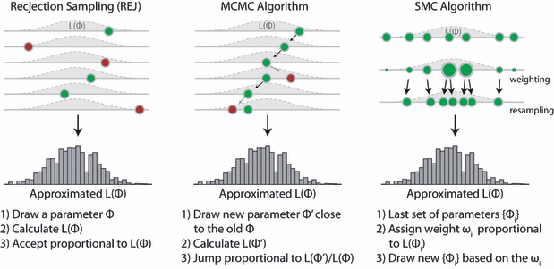
There is one disadvantage of this method that is obvious – you propose from the whole parameter space, which means that you will typically get a lot of rejections, which is costly (well, it’s called rejection sampling after all). MCMC, in contrast, does a random walk (Markov-chain) in parameter space, and thereby concentrates sampling on the important parameter areas. That is why it is more efficient. But MCMC also has a drawback – because the next step depends on the last step, it’s difficult to parallelize. SMC and rejection sampling, on the other hand, work in parallel anyway and are therefore trivially parallelizable. To see the difference to other sampling methods visually, have a look at this illustration of the three methods, taken from our 2011 EL review

Illustration of the three main classes of Monte-Carlo samplers

There are more benefits to rejection sampling than parallelization. For example when using rejection sampling for Approximate Bayesian Computation, there is the subtle but practically relevant advantage that you don’t have to choose the acceptance parameter in advance of the simulations. Finally, rejection sampling is a modern classic. I hope that’s enough motivation.

So, here is how you would do it in R:

An example in R

Assume we want to draw from a beta distribution with shape parameters 3,6, which looks like this

curve(dbeta(x, 3,6),0,1)

Target distribution

To do this, we first create a data.frame with 100000 random values between 0 and 1, and calculate their beta density values

sampled <- data.frame(proposal = runif(100000,0,1))
sampled$targetDensity <- dbeta(sampled$proposal, 3,6)

Now, accept proportional to the targetDensity. It’s easiest if we calculate the highest density value, and then accept the others in relation to that

maxDens = max(sampled$targetDensity, na.rm = T)
sampled$accepted = ifelse(runif(100000,0,1) < sampled$targetDensity / maxDens, TRUE, FALSE)

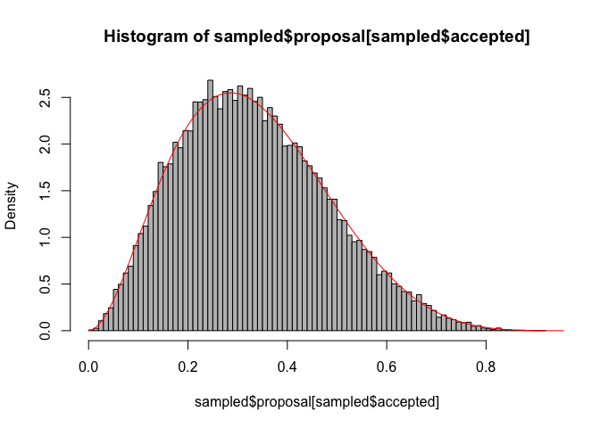
Plot the result

hist(sampled$proposal[sampled$accepted], freq = F, col = "grey", breaks = 100)
curve(dbeta(x, 3,6),0,1, add =T, col = "red")

Sample created by rejection sampling, and comparison to the target distribution

A copy of the entire code is available on GitHub here